Matrix Inverses, Cramer’s Rule & Linear Vector Spaces
Lecture Video
Background
We have previously studied how to solve systems of two equations by substitution or elimination. But what happens when one has five equations in five unknowns — or a hundred? Matrices provide a systematic way to handle this, and the inverse matrix yields the solution in one clean step: \(\mathbf{x} = M^{-1}\mathbf{f}\).
In this lesson we tie together several threads from previous sessions. First, we finish the proof of Cramer’s Rule by showing exactly why the numerator takes the form of a determinant with one column replaced. Then we prove a subtle but important fact: if \(M^{-1}M = I\), then \(M M^{-1} = I\) as well — the inverse works from both sides. Finally, we enter new territory: linear vector spaces. We define them rigorously, explore examples in 2D and 3D, and meet the kernel of a matrix — a concept that connects solutions of equations to the geometry of space.
- Cramer’s Rule (Numerator): The \(i\)th component of the solution is \(x_i = \frac{\det(M_i)}{\det(M)}\), where \(M_i\) is \(M\) with the \(i\)th column replaced by the constant vector \(\mathbf{f}\).
- Commutativity of Inverses: If \(M^{-1}M = I\), then \(MM^{-1} = I\) also holds — proved using the non-zero determinant of \(M\).
- Linear Vector Space: A set \(V\) is a linear vector space if it is closed under linear combination: for any \(\mathbf{v}_1, \mathbf{v}_2 \in V\) and scalars \(\alpha, \beta\), we have \(\alpha \mathbf{v}_1 + \beta \mathbf{v}_2 \in V\).
- The Kernel: \(\ker(M) = \{\mathbf{x} : M\mathbf{x} = \mathbf{0}\}\) is always a linear vector space.
- The Range: \(\text{range}(M) = \{\mathbf{w} : \mathbf{w} = M\mathbf{u} \text{ for some } \mathbf{u}\}\) is also a linear vector space (homework to prove).
Completing Cramer’s Rule: Where the Numerator Comes From
Recall the setup. We have a system \(M\mathbf{x} = \mathbf{f}\), where:
\[M = \begin{pmatrix} m_{11} & m_{12} & \cdots & m_{1n} \\ m_{21} & m_{22} & \cdots & m_{2n} \\ \vdots & & \ddots & \vdots \\ m_{n1} & m_{n2} & \cdots & m_{nn} \end{pmatrix}, \quad \mathbf{f} = \begin{pmatrix} f_1 \\ f_2 \\ \vdots \\ f_n \end{pmatrix}\]
The solution is \(\mathbf{x} = M^{-1}\mathbf{f}\), where the inverse matrix is built from cofactors:
\[(M^{-1})_{ij} = \frac{(-1)^{i+j} \, \mathcal{M}_{ji}}{\det(M)}\]
Here \(\mathcal{M}_{ji}\) is the minor (the determinant of the submatrix obtained by deleting row \(j\) and column \(i\)).
Multiplying Out \(x_1\)
To find \(x_1\), multiply the first row of \(M^{-1}\) by \(\mathbf{f}\):
\[x_1 = \frac{1}{\det(M)}\bigl(\mathcal{M}_{11}\,f_1 - \mathcal{M}_{21}\,f_2 + \mathcal{M}_{31}\,f_3 - \cdots + (-1)^{n+1}\mathcal{M}_{n1}\,f_n\bigr)\]
Look at the expression in parentheses. Each \(\mathcal{M}_{k1}\) is the cofactor associated with the element in row \(k\), column \(1\) of the original matrix. But instead of multiplying each cofactor by \(m_{k1}\) (the original first-column entry), we are multiplying by \(f_k\).
This is exactly the cofactor expansion along the first column of a modified matrix — the matrix \(M\) with its first column replaced by \(\mathbf{f}\):
\[M_1 = \begin{pmatrix} f_1 & m_{12} & \cdots & m_{1n} \\ f_2 & m_{22} & \cdots & m_{2n} \\ \vdots & & \ddots & \vdots \\ f_n & m_{n2} & \cdots & m_{nn} \end{pmatrix}\]
The cofactors \(\mathcal{M}_{k1}\) are unchanged because they come from deleting row \(k\) and column \(1\) — and we only changed column \(1\). So the numerator is \(\det(M_1)\), and we arrive at:
\[\boxed{x_i = \frac{\det(M_i)}{\det(M)}}\]
where \(M_i\) has the \(i\)th column of \(M\) replaced by \(\mathbf{f}\). This is Cramer’s Rule.
Solve \(\begin{cases} 3x + 2y = 7 \\ x - y = 1 \end{cases}\)
Here \(M = \begin{pmatrix} 3 & 2 \\ 1 & -1 \end{pmatrix}\) and \(\mathbf{f} = \begin{pmatrix} 7 \\ 1 \end{pmatrix}\).
\[\det(M) = 3(-1) - 2(1) = -5\]
\[x = \frac{\det\begin{pmatrix} 7 & 2 \\ 1 & -1 \end{pmatrix}}{\det(M)} = \frac{7(-1) - 2(1)}{-5} = \frac{-9}{-5} = \frac{9}{5}\]
\[y = \frac{\det\begin{pmatrix} 3 & 7 \\ 1 & 1 \end{pmatrix}}{\det(M)} = \frac{3(1) - 7(1)}{-5} = \frac{-4}{-5} = \frac{4}{5}\]
Check: \(3(9/5) + 2(4/5) = 27/5 + 8/5 = 35/5 = 7\) and \(9/5 - 4/5 = 5/5 = 1\).
Proving \(M^{-1}M = I \implies MM^{-1} = I\)
Matrix multiplication is not commutative in general: \(AB \neq BA\). So it is not obvious that if \(M^{-1}M = I\) (left inverse), then \(MM^{-1} = I\) (right inverse). Here is the elegant proof developed in class.
The Setup
We know \(M^{-1}M = I\). Define the unknown matrix:
\[X = MM^{-1}\]
We want to show \(X = I\).
Step 1: Discover a Property of \(X\)
Right-multiply \(X\) by \(M\):
\[XM = (MM^{-1})M = M(M^{-1}M) = MI = M\]
using the associativity of matrix multiplication. So we know:
\[XM = M\]
Rearranging:
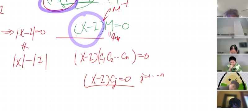
\[(X - I)M = 0\]
Step 2: Why \((X - I)\) Must Be the Zero Matrix
The equation \((X - I)M = 0\) says that the matrix \((X - I)\) sends every column of \(M\) to the zero vector. Let \(\mathbf{c}_1, \mathbf{c}_2, \ldots, \mathbf{c}_n\) be the columns of \(M\):
\[(X - I)\mathbf{c}_j = \mathbf{0} \quad \text{for } j = 1, 2, \ldots, n\]
Since \(\det(M) \neq 0\), the columns of \(M\) are linearly independent — they span the entire \(n\)-dimensional space. Any vector \(\mathbf{v}\) can be written as a linear combination \(\mathbf{v} = \alpha_1 \mathbf{c}_1 + \cdots + \alpha_n \mathbf{c}_n\).
By linearity:
\[(X - I)\mathbf{v} = \alpha_1 (X - I)\mathbf{c}_1 + \cdots + \alpha_n (X - I)\mathbf{c}_n = \alpha_1 \mathbf{0} + \cdots + \alpha_n \mathbf{0} = \mathbf{0}\]
Since \((X - I)\mathbf{v} = \mathbf{0}\) for every vector \(\mathbf{v}\), the matrix \(X - I\) must be the zero matrix.
Lucas’s method (test with \(I\)): Choose \(\mathbf{v}\) to be each standard basis vector \(\mathbf{e}_1 = (1,0,\ldots,0)^T\), \(\mathbf{e}_2 = (0,1,\ldots,0)^T\), etc. Then \((X - I)\mathbf{e}_j\) extracts the \(j\)th column of \(X - I\), which must be zero. All \(n\) columns are zero, so \(X - I = 0\).
Toby’s method (proof by contradiction): Suppose some entry \((X - I)_{ij} \neq 0\). Choose \(\mathbf{v} = \mathbf{e}_j\) (the vector with a \(1\) in position \(j\) and zeros elsewhere). Then \((X - I)\mathbf{e}_j\) has a nonzero entry in row \(i\) — contradicting \((X - I)\mathbf{v} = \mathbf{0}\).
Both methods crucially use the fact that \(\det(M) \neq 0\), which guarantees the columns of \(M\) span \(\mathbb{R}^n\).
\[\boxed{X - I = 0 \implies MM^{-1} = I}\]
Linear Vector Spaces
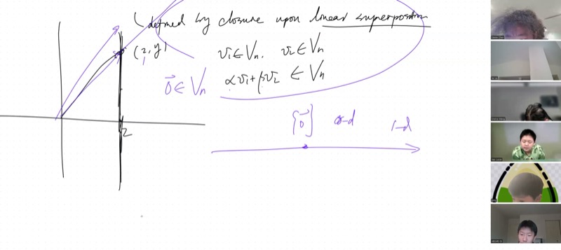
A linear vector space \(V_n\) is a set of vectors that is closed under linear combination:
\[\text{For all } \mathbf{v}_1, \mathbf{v}_2 \in V_n \text{ and all scalars } \alpha, \beta \in \mathbb{R}: \quad \alpha\mathbf{v}_1 + \beta\mathbf{v}_2 \in V_n\]
This single condition automatically guarantees:
- Scaling: Setting \(\beta = 0\) gives \(\alpha\mathbf{v}_1 \in V_n\)
- Zero vector: Setting \(\alpha = \beta = 0\) gives \(\mathbf{0} \in V_n\)
- Addition: Setting \(\alpha = \beta = 1\) gives \(\mathbf{v}_1 + \mathbf{v}_2 \in V_n\)
Examples and Non-Examples
No. Take two vectors on this line: \(\mathbf{v}_1 = (2, 0)\) and \(\mathbf{v}_2 = (2, 5)\). Scale \(\mathbf{v}_1\) by \(3\): you get \((6, 0)\), which has \(x = 6 \neq 2\) — it leaves the line.
Also, the zero vector \((0, 0)\) has \(x = 0 \neq 2\), so it is not in the set. A line must pass through the origin to be a vector space.
Yes. Any two vectors in the plane can be added (parallelogram rule) and scaled, and the result stays in the plane. The plane is a 2-dimensional linear vector space, even though it sits inside 3D space.
A plane not through the origin fails: it does not contain \(\mathbf{0}\).
Hierarchy of Linear Vector Spaces
| Dimension | Description | Number of Elements |
|---|---|---|
| \(0\) | Just the zero vector \(\{\mathbf{0}\}\) | \(1\) |
| \(1\) | A line through the origin | \(\infty\) |
| \(2\) | A plane through the origin | \(\infty\) |
| \(n\) | The full \(n\)-dimensional space \(\mathbb{R}^n\) | \(\infty\) |
The smallest linear vector space has a single element: \(\{\mathbf{0}\}\). Every other linear vector space has infinitely many elements.
Affine Coordinates and Non-Orthogonal Bases
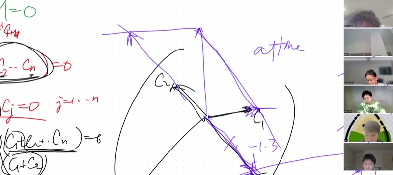
If two vectors \(\mathbf{c}_1\) and \(\mathbf{c}_2\) are linearly independent (not parallel), they span the 2D plane. Any vector \(\mathbf{v}\) in the plane can be decomposed as:
\[\mathbf{v} = \alpha \mathbf{c}_1 + \beta \mathbf{c}_2\]
The coefficients \((\alpha, \beta)\) are the affine coordinates of \(\mathbf{v}\) with respect to the basis \(\{\mathbf{c}_1, \mathbf{c}_2\}\). The grid lines form a parallelogram grid rather than a rectangular one, but every point is still uniquely determined.
The Kernel of a Matrix
Definition. The kernel (or null space) of a matrix \(M\) is the set of all vectors that \(M\) maps to zero:
\[\ker(M) = \{\mathbf{x} \in \mathbb{R}^n : M\mathbf{x} = \mathbf{0}\}\]
Let \(\mathbf{x}_1, \mathbf{x}_2 \in \ker(M)\), so \(M\mathbf{x}_1 = \mathbf{0}\) and \(M\mathbf{x}_2 = \mathbf{0}\).
For any scalars \(\alpha, \beta\):
\[M(\alpha\mathbf{x}_1 + \beta\mathbf{x}_2) = \alpha M\mathbf{x}_1 + \beta M\mathbf{x}_2 = \alpha\mathbf{0} + \beta\mathbf{0} = \mathbf{0}\]
Therefore \(\alpha\mathbf{x}_1 + \beta\mathbf{x}_2 \in \ker(M)\).
The key step uses the linearity of matrix multiplication: \(M(\alpha\mathbf{u} + \beta\mathbf{v}) = \alpha M\mathbf{u} + \beta M\mathbf{v}\).
Two Cases for the Kernel
| Condition | Kernel |
|---|---|
| \(\det(M) \neq 0\) (invertible) | \(\ker(M) = \{\mathbf{0}\}\) — only the trivial solution, a 0-dimensional space |
| \(\det(M) = 0\) (singular) | \(\ker(M)\) contains nontrivial solutions — dimension \(\geq 1\) |
When \(\det(M) = 0\), the columns of \(M\) are linearly dependent, and there is a whole subspace of vectors that \(M\) collapses to zero.
The Range of a Matrix (Homework)
Definition. The range (or column space) of \(M\) is the set of all vectors that can be expressed as \(M\mathbf{u}\) for some \(\mathbf{u}\):
\[\text{range}(M) = \{\mathbf{w} : \mathbf{w} = M\mathbf{u} \text{ for some } \mathbf{u} \in \mathbb{R}^n\}\]
Prove that \(\text{range}(M)\) is a linear vector space. Hint: Follow the same approach as the kernel proof. Take two vectors \(\mathbf{w}_1 = M\mathbf{u}_1\) and \(\mathbf{w}_2 = M\mathbf{u}_2\) in the range, and show that \(\alpha\mathbf{w}_1 + \beta\mathbf{w}_2\) is also in the range.
Key Video Frames

Cheat Sheet
| Concept | Formula / Rule |
|---|---|
| Cramer’s Rule | \(x_i = \dfrac{\det(M_i)}{\det(M)}\), where \(M_i\) has column \(i\) replaced by \(\mathbf{f}\) |
| Inverse Matrix | \((M^{-1})_{ij} = \dfrac{(-1)^{i+j}\,\mathcal{M}_{ji}}{\det(M)}\) (cofactors, transposed) |
| Inverse Commutativity | \(M^{-1}M = I \iff MM^{-1} = I\) (requires \(\det(M) \neq 0\)) |
| Linear Vector Space | Closed under \(\alpha\mathbf{v}_1 + \beta\mathbf{v}_2\) for all scalars \(\alpha, \beta\) |
| Must contain \(\mathbf{0}\) | Set \(\alpha = \beta = 0\) in the closure condition |
| Kernel | \(\ker(M) = \{\mathbf{x} : M\mathbf{x} = \mathbf{0}\}\) — always a linear vector space |
| Range | \(\text{range}(M) = \{M\mathbf{u} : \mathbf{u} \in \mathbb{R}^n\}\) — always a linear vector space |
| Linear Independence | \(\det(M) \neq 0 \iff\) columns of \(M\) span all of \(\mathbb{R}^n\) |
| Affine Coordinates | Any \(\mathbf{v} = \alpha\mathbf{c}_1 + \beta\mathbf{c}_2\) when \(\mathbf{c}_1, \mathbf{c}_2\) are linearly independent |
| Smallest vector space | \(\{\mathbf{0}\}\) (zero-dimensional, one element) |
Quick Reference: Key Properties of Invertible Matrices
| Property | Consequence |
|---|---|
| \(\det(M) \neq 0\) | \(M\) is invertible |
| \(M^{-1}\) exists | \(M\mathbf{x} = \mathbf{f}\) has a unique solution \(\mathbf{x} = M^{-1}\mathbf{f}\) |
| Columns are linearly independent | They span \(\mathbb{R}^n\) and form a basis |
| \(\ker(M) = \{\mathbf{0}\}\) | Only the trivial solution to \(M\mathbf{x} = \mathbf{0}\) |
| \(\det(AB) = \det(A)\det(B)\) | Determinant of a product is the product of determinants |