Eigenvalues, Eigenvectors & Orthogonal Matrix Diagonalization

Lecture Video

Background

Imagine you have a quadratic expression like \(3x^2 + 4xy + y^2\). This looks messy because of the \(xy\) cross-term — you cannot immediately tell whether this equation describes an ellipse, a hyperbola, or a parabola. But what if you could rotate your coordinate axes so the cross-term disappears, leaving you with something clean like \(\lambda_1 u^2 + \lambda_2 v^2\)?

That is exactly what matrix diagonalization achieves. Every symmetric matrix can be “unscrambled” by a rotation into a diagonal matrix whose entries — the eigenvalues — reveal the true geometry hiding inside the original expression. The rotation directions are given by eigenvectors, and the rotation matrix is an orthogonal matrix whose inverse is simply its transpose.

This lesson pulls together the threads from previous sessions: the quadratic form, rotational matrices, the tangent formula for finding the rotation angle, and two powerful invariants (the trace and the determinant) that let you find eigenvalues without computing the rotation at all. By the end, you will see how the equation \(M\vec{\varepsilon} = \lambda\vec{\varepsilon}\) defines eigenvalues and eigenvectors — one of the most important equations in all of mathematics and physics.

ImportantKey Ideas

1. Quadratic Form as a Matrix: The expression \(ax^2 + 2bxy + cy^2\) is encoded in the symmetric matrix \(\begin{pmatrix} a & b \\ b & c \end{pmatrix}\), called a metric tensor.
2. Diagonalization by Rotation: A symmetric \(2 \times 2\) matrix can always be diagonalized: \(M = R(-\theta)\begin{pmatrix}\lambda_1 & 0 \\ 0 & \lambda_2\end{pmatrix}R(\theta)\), where \(R(\theta)\) is a rotation matrix.
3. Two Invariants Find Eigenvalues: The trace \(\lambda_1 + \lambda_2 = a + c\) and the determinant \(\lambda_1 \lambda_2 = ac - b^2\) are unchanged by rotation, so you can find \(\lambda_1, \lambda_2\) without computing \(\theta\).
4. Orthogonal Matrices: A matrix whose columns are orthonormal vectors satisfies \(O^T O = I\), meaning \(O^{-1} = O^T\). Rotation matrices are orthogonal.
5. Eigenvalue Equation: The fundamental relationship \(M\vec{\varepsilon} = \lambda\vec{\varepsilon}\) says that multiplying the eigenvector \(\vec{\varepsilon}\) by \(M\) simply scales it by the eigenvalue \(\lambda\).

From Quadratic Forms to Matrices

Every quadratic expression in two variables can be written using a symmetric matrix:

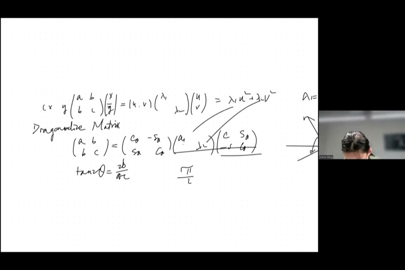
\[ax^2 + 2bxy + cy^2 = \begin{pmatrix} x & y \end{pmatrix} \begin{pmatrix} a & b \\ b & c \end{pmatrix} \begin{pmatrix} x \\ y \end{pmatrix}\]

This matrix \(M = \begin{pmatrix} a & b \\ b & c \end{pmatrix}\) is called a metric tensor — it encodes a “twisted” way of measuring distance. In ordinary Euclidean geometry, distance is \(x^2 + y^2\) (the Pythagorean sum). A general metric allows weighted and mixed terms.

TipExample: Identifying the Conic from a Quadratic

Consider \(2x^2 + 6xy + 5y^2 = 1\). The matrix is:

\[M = \begin{pmatrix} 2 & 3 \\ 3 & 5 \end{pmatrix}\]

To classify this conic, we find the eigenvalues using our two invariants:

• Trace: \(\lambda_1 + \lambda_2 = 2 + 5 = 7\)
• Determinant: \(\lambda_1 \lambda_2 = (2)(5) - 3^2 = 1\)

So \(\lambda_1\) and \(\lambda_2\) satisfy \(\lambda^2 - 7\lambda + 1 = 0\), giving \(\lambda = \frac{7 \pm \sqrt{45}}{2} = \frac{7 \pm 3\sqrt{5}}{2}\).

Both eigenvalues are positive, so the conic is an ellipse.

When Eigenvalues Have Different Signs

The sign pattern of \(\lambda_1, \lambda_2\) determines the conic section:

Eigenvalue signs	Conic type	Example metric
Both positive	Ellipse	Standard distance
Both negative	Ellipse (reflected)	Negative-definite
Opposite signs	Hyperbola	Minkowski metric (\(\lambda_1 = 1, \lambda_2 = -1\))
One is zero	Parabola	Degenerate case

In Einstein’s theory of relativity, spacetime uses the Minkowski metric with \(\lambda_1 = 1\) and \(\lambda_2 = -1\). This gives rise to hyperbolic geometry, where the “distance” \(t^2 - x^2\) can be negative — profoundly different from everyday Euclidean geometry, yet governing the fabric of our universe.

Diagonalization: Two Routes to Eigenvalues

There are two approaches to diagonalizing the matrix \(M = \begin{pmatrix} a & b \\ b & c \end{pmatrix}\).

Route 1: Find the Rotation Angle First

From the previous session, the rotation angle \(\theta\) that eliminates the cross-term satisfies:

\[\tan(2\theta) = \frac{2b}{a - c}\]

This equation has period \(\pi\) in \(2\theta\), so \(\theta\) has period \(\frac{\pi}{2}\). If \(\theta\) is a solution, then \(\theta + \frac{\pi}{2}\) is also a solution — which makes sense, because swapping the two axes (a 90-degree rotation) just exchanges \(\lambda_1\) and \(\lambda_2\).

After finding \(\theta\), you compute \(\cos\theta\) and \(\sin\theta\), plug into the rotated matrix, and read off \(\lambda_1, \lambda_2\). This works but involves a lot of trigonometric algebra.

Route 2: Use Invariants (Skip the Angle!)

A much cleaner approach uses two quantities that do not change under rotation:

\[\boxed{\lambda_1 + \lambda_2 = a + c \qquad \text{(trace)}}\]

\[\boxed{\lambda_1 \lambda_2 = ac - b^2 \qquad \text{(determinant)}}\]

These two equations let you solve for \(\lambda_1\) and \(\lambda_2\) directly — no trigonometry required. They are the roots of the characteristic polynomial:

\[\lambda^2 - (a+c)\lambda + (ac - b^2) = 0\]

Adjust the sliders for \(a\), \(b\), \(c\) above to see how different matrix entries change the conic. When the determinant \(ac - b^2\) is positive, you get an ellipse; when negative, a hyperbola.

TipExample: Finding Eigenvalues via Invariants

Given \(M = \begin{pmatrix} 5 & 2 \\ 2 & 1 \end{pmatrix}\):

Trace: \(\lambda_1 + \lambda_2 = 5 + 1 = 6\)

Determinant: \(\lambda_1 \lambda_2 = 5 \cdot 1 - 2^2 = 1\)

Characteristic polynomial: \(\lambda^2 - 6\lambda + 1 = 0\)

\[\lambda = \frac{6 \pm \sqrt{36 - 4}}{2} = \frac{6 \pm \sqrt{32}}{2} = 3 \pm 2\sqrt{2}\]

So \(\lambda_1 = 3 + 2\sqrt{2} \approx 5.83\) and \(\lambda_2 = 3 - 2\sqrt{2} \approx 0.17\). Both positive, so the quadratic form defines an ellipse.

Proving the Trace Invariant

When you write out the diagonalization:

\[\begin{pmatrix} a & b \\ b & c \end{pmatrix} = \begin{pmatrix} \cos\theta & \sin\theta \\ -\sin\theta & \cos\theta \end{pmatrix} \begin{pmatrix} \lambda_1 & 0 \\ 0 & \lambda_2 \end{pmatrix} \begin{pmatrix} \cos\theta & -\sin\theta \\ \sin\theta & \cos\theta \end{pmatrix}\]

and multiply everything out, you find:

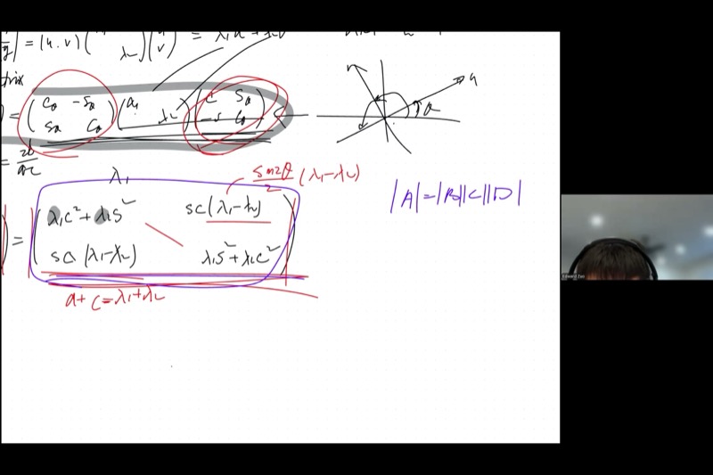
\[a = \lambda_1 \cos^2\theta + \lambda_2 \sin^2\theta\] \[c = \lambda_1 \sin^2\theta + \lambda_2 \cos^2\theta\]

Adding these:

\[a + c = \lambda_1(\cos^2\theta + \sin^2\theta) + \lambda_2(\sin^2\theta + \cos^2\theta) = \lambda_1 + \lambda_2\]

The Pythagorean identity \(\cos^2\theta + \sin^2\theta = 1\) causes \(\theta\) to vanish completely. The trace is invariant under rotation.

Proving the Determinant Invariant

NoteFull Calculation: Determinant Is Invariant

We compute the determinant of the expanded matrix directly. After multiplying out:

\[a = \lambda_1\cos^2\theta + \lambda_2\sin^2\theta, \quad c = \lambda_1\sin^2\theta + \lambda_2\cos^2\theta\] \[b = (\lambda_1 - \lambda_2)\sin\theta\cos\theta\]

The determinant \(ac - b^2\):

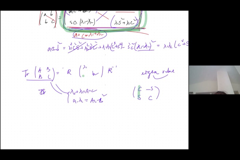
Product \(ac\): \[ac = (\lambda_1\cos^2\theta + \lambda_2\sin^2\theta)(\lambda_1\sin^2\theta + \lambda_2\cos^2\theta)\]

Expanding:

\[= \lambda_1^2 \cos^2\theta\sin^2\theta + \lambda_1\lambda_2\cos^4\theta + \lambda_1\lambda_2\sin^4\theta + \lambda_2^2\sin^2\theta\cos^2\theta\]

\[= (\lambda_1^2 + \lambda_2^2)\cos^2\theta\sin^2\theta + \lambda_1\lambda_2(\cos^4\theta + \sin^4\theta)\]

Term \(b^2\): \[b^2 = (\lambda_1 - \lambda_2)^2 \sin^2\theta\cos^2\theta\]

Subtraction \(ac - b^2\):

\[= \lambda_1\lambda_2(\cos^4\theta + \sin^4\theta) + [(\lambda_1^2 + \lambda_2^2) - (\lambda_1 - \lambda_2)^2]\sin^2\theta\cos^2\theta\]

Now \((\lambda_1^2 + \lambda_2^2) - (\lambda_1 - \lambda_2)^2 = 2\lambda_1\lambda_2\), so:

\[= \lambda_1\lambda_2(\cos^4\theta + \sin^4\theta + 2\sin^2\theta\cos^2\theta)\]

\[= \lambda_1\lambda_2(\cos^2\theta + \sin^2\theta)^2 = \lambda_1\lambda_2\]

The angle vanishes completely, confirming \(\det M = \lambda_1\lambda_2\).

Geometric Intuition: Why the Determinant Is Invariant

The determinant measures the area (or volume) of the parallelogram spanned by the matrix’s column vectors. A rotation does not stretch or compress anything — it only turns. Since the two rotation matrices each have determinant \(1\), the overall scaling factor is \(1 \times \lambda_1\lambda_2 \times 1 = \lambda_1\lambda_2\).

This is the factorization theorem for determinants: \(\det(ABC) = \det(A)\det(B)\det(C)\). While we verified it by direct computation in this case, the general theorem is a deep result that requires more advanced linear algebra to prove rigorously.

Orthogonal Matrices and Eigenvectors

The Rotation Matrix as a Pair of Vectors

The rotation matrix can be viewed as two column vectors:

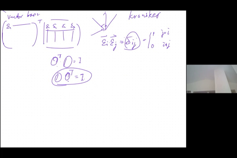
\[R(\theta) = \begin{pmatrix} \cos\theta & -\sin\theta \\ \sin\theta & \cos\theta \end{pmatrix} = \begin{pmatrix} | & | \\ \vec{\varepsilon}_1 & \vec{\varepsilon}_2 \\ | & | \end{pmatrix}\]

where \(\vec{\varepsilon}_1 = \begin{pmatrix}\cos\theta \\ \sin\theta\end{pmatrix}\) and \(\vec{\varepsilon}_2 = \begin{pmatrix}-\sin\theta \\ \cos\theta\end{pmatrix}\).

These vectors have three remarkable properties:

1. Unit length: \(|\vec{\varepsilon}_1| = |\vec{\varepsilon}_2| = 1\) (by the Pythagorean identity)
2. Orthogonal: \(\vec{\varepsilon}_1 \cdot \vec{\varepsilon}_2 = \cos\theta(-\sin\theta) + \sin\theta\cos\theta = 0\)
3. Negative reciprocal slopes: slope of \(\vec{\varepsilon}_1\) is \(\frac{\sin\theta}{\cos\theta} = \tan\theta\); slope of \(\vec{\varepsilon}_2\) is \(\frac{\cos\theta}{-\sin\theta} = -\cot\theta = -\frac{1}{\tan\theta}\)

Together, \(\vec{\varepsilon}_1\) and \(\vec{\varepsilon}_2\) form an orthonormal basis — a rotated version of the standard \(\hat{i}, \hat{j}\) directions.

Drag the \(\theta_0\) slider to rotate the orthonormal basis \(\vec{\varepsilon}_1\) (blue) and \(\vec{\varepsilon}_2\) (red). They always remain perpendicular and unit-length.

The Orthogonal Matrix Property

A matrix \(O\) built from orthonormal column vectors is called an orthogonal matrix. Its defining property is:

\[\boxed{O^T O = I \qquad \Longleftrightarrow \qquad O^{-1} = O^T}\]

Why this works: When you multiply \(O^T O\), the \((i,j)\) entry is the dot product \(\vec{\varepsilon}_i \cdot \vec{\varepsilon}_j\). Since the columns are orthonormal:

\[\vec{\varepsilon}_i \cdot \vec{\varepsilon}_j = \delta_{ij} = \begin{cases} 1 & \text{if } i = j \\ 0 & \text{if } i \neq j \end{cases}\]

This is the Kronecker delta — it produces the identity matrix.

NoteProof: Left Inverse Implies Right Inverse

We proved \(O^T O = I\), but does \(O O^T = I\) also hold?

Starting from \(O^T O = I\), multiply both sides on the right by \(O^T\):

\[O^T O \cdot O^T = O^T\] \[O^T (O O^T - I) = 0\]

Since \(O^T\) has full rank (its determinant is nonzero — it is built from independent vectors), the only matrix \(X\) satisfying \(O^T X = 0\) is \(X = 0\). Therefore:

\[O O^T - I = 0 \qquad \Longrightarrow \qquad O O^T = I\]

A left inverse of an orthogonal matrix is also its right inverse.

Higher Dimensions

This structure generalizes naturally. In \(n\) dimensions, an orthogonal matrix \(O\) is built from \(n\) mutually orthogonal unit vectors \(\vec{\varepsilon}_1, \vec{\varepsilon}_2, \ldots, \vec{\varepsilon}_n\). The property \(O^T O = I\) still holds, and \(O^{-1} = O^T\) remains true. The Kronecker delta encodes all the pairwise dot products:

\[\vec{\varepsilon}_i \cdot \vec{\varepsilon}_j = \delta_{ij} \quad \text{for all } i, j = 1, \ldots, n\]

The Eigenvalue Equation

Now we reach the culmination. Starting from the diagonalization:

\[M = E \begin{pmatrix} \lambda_1 & 0 \\ 0 & \lambda_2 \end{pmatrix} E^T\]

where \(E = \begin{pmatrix} \vec{\varepsilon}_1 & \vec{\varepsilon}_2 \end{pmatrix}\) is the orthogonal matrix of eigenvectors, multiply both sides on the right by \(E\):

\[M E = E \begin{pmatrix} \lambda_1 & 0 \\ 0 & \lambda_2 \end{pmatrix}\]

since \(E^T E = I\). Written as column vectors:

\[M \begin{pmatrix} \vec{\varepsilon}_1 & \vec{\varepsilon}_2 \end{pmatrix} = \begin{pmatrix} \vec{\varepsilon}_1 & \vec{\varepsilon}_2 \end{pmatrix} \begin{pmatrix} \lambda_1 & 0 \\ 0 & \lambda_2 \end{pmatrix}\]

Multiply out the right-hand side column by column:

\[\begin{pmatrix} \vec{\varepsilon}_1 & \vec{\varepsilon}_2 \end{pmatrix} \begin{pmatrix} \lambda_1 & 0 \\ 0 & \lambda_2 \end{pmatrix} = \begin{pmatrix} \lambda_1 \vec{\varepsilon}_1 & \lambda_2 \vec{\varepsilon}_2 \end{pmatrix}\]

Comparing column by column, we get two separate equations:

\[\boxed{M\vec{\varepsilon}_1 = \lambda_1 \vec{\varepsilon}_1 \qquad \text{and} \qquad M\vec{\varepsilon}_2 = \lambda_2 \vec{\varepsilon}_2}\]

This is the eigenvalue equation: multiplying the matrix \(M\) by an eigenvector \(\vec{\varepsilon}\) simply scales the vector by its corresponding eigenvalue \(\lambda\). The matrix does not rotate or distort the eigenvector — it only stretches (or compresses or reflects) it.

TipExample: Verify the Eigenvalue Equation

For \(M = \begin{pmatrix} 3 & 1 \\ 1 & 3 \end{pmatrix}\):

Eigenvalues: trace \(= 6\), determinant \(= 9 - 1 = 8\), so \(\lambda^2 - 6\lambda + 8 = 0\), giving \(\lambda_1 = 4\), \(\lambda_2 = 2\).

Finding \(\vec{\varepsilon}_1\) for \(\lambda_1 = 4\): Solve \((M - 4I)\vec{v} = \vec{0}\):

\[\begin{pmatrix} -1 & 1 \\ 1 & -1 \end{pmatrix}\begin{pmatrix} v_1 \\ v_2 \end{pmatrix} = \begin{pmatrix} 0 \\ 0 \end{pmatrix} \implies v_1 = v_2\]

Normalized: \(\vec{\varepsilon}_1 = \frac{1}{\sqrt{2}}\begin{pmatrix} 1 \\ 1 \end{pmatrix}\)

Verify: \(M\vec{\varepsilon}_1 = \begin{pmatrix} 3 & 1 \\ 1 & 3 \end{pmatrix}\frac{1}{\sqrt{2}}\begin{pmatrix} 1 \\ 1 \end{pmatrix} = \frac{1}{\sqrt{2}}\begin{pmatrix} 4 \\ 4 \end{pmatrix} = 4 \cdot \frac{1}{\sqrt{2}}\begin{pmatrix} 1 \\ 1 \end{pmatrix} = 4\vec{\varepsilon}_1\)

Similarly, \(\vec{\varepsilon}_2 = \frac{1}{\sqrt{2}}\begin{pmatrix} 1 \\ -1 \end{pmatrix}\) is the eigenvector for \(\lambda_2 = 2\).

Non-Zero Product of Matrices Can Be Zero

An interesting aside from the lecture: can two nonzero matrices multiply to give the zero matrix?

Yes. For example:

\[\begin{pmatrix} 1 & 0 \\ 0 & 0 \end{pmatrix} \begin{pmatrix} 0 & 0 \\ 0 & 1 \end{pmatrix} = \begin{pmatrix} 0 & 0 \\ 0 & 0 \end{pmatrix}\]

Neither factor is zero, but their product is. This happens because one matrix “projects” onto dimensions that the other annihilates. However, if a matrix has full rank (nonzero determinant, all columns linearly independent), then \(AX = 0\) forces \(X = 0\). This is why orthogonal matrices — which always have determinant \(\pm 1\) — can never produce such cancellation.

Key Video Frames

Cheat Sheet

Concept	Formula / Rule
Symmetric matrix	\(M = \begin{pmatrix} a & b \\ b & c \end{pmatrix}\) encodes the quadratic \(ax^2 + 2bxy + cy^2\)
Rotation angle	\(\tan(2\theta) = \dfrac{2b}{a - c}\)
Trace (sum of diagonal)	\(\operatorname{tr}(M) = a + c = \lambda_1 + \lambda_2\)
Determinant	\(\det(M) = ac - b^2 = \lambda_1\lambda_2\)
Characteristic polynomial	\(\lambda^2 - (a+c)\lambda + (ac - b^2) = 0\)
Eigenvalue equation	\(M\vec{\varepsilon} = \lambda\vec{\varepsilon}\)
Orthogonal matrix	\(O^T O = O O^T = I\), so \(O^{-1} = O^T\)
Kronecker delta	\(\vec{\varepsilon}_i \cdot \vec{\varepsilon}_j = \delta_{ij}\)
Conic classification	Same-sign \(\lambda\): ellipse; opposite signs: hyperbola; one zero: parabola
Minkowski metric	\(\lambda_1 = 1, \lambda_2 = -1\) gives spacetime hyperbolic geometry

Quick Reference: Diagonalization Steps

Step	Action
1	Compute trace: \(\lambda_1 + \lambda_2 = a + c\)
2	Compute determinant: \(\lambda_1\lambda_2 = ac - b^2\)
3	Solve \(\lambda^2 - \operatorname{tr}\lambda + \det = 0\) for eigenvalues
4	Classify conic from signs of \(\lambda_1, \lambda_2\)
5	(Optional) Find \(\theta\) from \(\tan(2\theta) = 2b/(a-c)\) for the rotation
6	Find eigenvectors by solving \((M - \lambda I)\vec{v} = \vec{0}\)