Linear Recurrences: Double Roots, Generating Functions & Summing Scaled Geometric Series
Linear recurrences arise whenever the next value in a sequence depends on previous values – population models, compound interest, computer algorithms, and signal processing all rely on them. The Fibonacci sequence is a famous example, and the techniques in this lesson let you solve any second-order linear recurrence in closed form.
Topics Covered
- Solving second-order linear recurrences via the characteristic equation
- The double root case: why a single exponential term is not enough
- Degrees of freedom and fitting initial conditions
- Telescoping sums to recover the general formula
- Generating functions and power series expansions
- Summing linearly-scaled geometric series: \(\sum (n+1) r^n\)
- Binomial expansion to negative powers
- Connection to Pascal’s triangle and higher powers of \(\frac{1}{1-x}\)
Lecture Video
Key Video Frames
Background: Second-Order Linear Recurrences
A second-order linear recurrence is a rule that defines each term using the two preceding terms:
\[f(n+1) = p \cdot f(n) + q \cdot f(n-1)\]
together with two initial conditions \(f(0)\) and \(f(1)\).
The recurrence is linear because \(f(n)\) and \(f(n-1)\) appear only to the first power – no \(f(n)^2\) or \(f(n) \cdot f(n-1)\) terms. This is what makes the characteristic equation method work.
The Characteristic Equation Method
- Characteristic equation: Replace \(f(n+1) = p\,f(n) + q\,f(n-1)\) with \(x^2 = px + q\), i.e., \(x^2 - px - q = 0\).
- Distinct roots \(x_1 \neq x_2\): The general solution is \(f(n) = A\,x_1^n + B\,x_2^n\).
- Double root \(x_1 = x_2 = r\): The general solution is \(f(n) = (A + Bn)\,r^n\).
- Two degrees of freedom (\(A\) and \(B\)) are always needed to fit the two initial conditions \(f(0)\) and \(f(1)\).
- Generating functions provide an alternative approach: encode the entire sequence as a power series and use partial fractions.
Step 1: From Recurrence to Characteristic Equation
Consider the running example from the lecture:
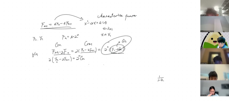
\[f(n+1) = 4\,f(n) - 4\,f(n-1)\]
We guess solutions of the form \(f(n) = x^n\). Substituting:
\[x^{n+1} = 4x^n - 4x^{n-1}\]
Dividing through by \(x^{n-1}\) (assuming \(x \neq 0\)):
\[x^2 - 4x + 4 = 0\]
Exponential solutions are natural for linear recurrences, just as \(e^{rx}\) is natural for linear differential equations. The recurrence says “the next term is a fixed linear combination of previous terms,” and geometric sequences \(x^n\) are exactly the sequences where ratios between consecutive terms are constant.
Step 2: Solving the Characteristic Equation
\[x^2 - 4x + 4 = (x - 2)^2 = 0\]
This gives a double root \(x_1 = x_2 = 2\).
Step 3: Why One Exponential Is Not Enough
If we tried \(f(n) = A \cdot 2^n\) as our general solution, we would have only one free parameter \(A\). But we need to satisfy two initial conditions:
- \(f(0) = A \cdot 2^0 = A\)
- \(f(1) = A \cdot 2^1 = 2A\)
Once \(f(0)\) is chosen, \(f(1)\) is forced to be \(2 \cdot f(0)\). But the recurrence allows any pair \((f(0), f(1))\)! For instance, \(f(0) = 1\) and \(f(1) = 4\) cannot be accommodated by \(f(n) = A \cdot 2^n\) alone.
We need a second independent parameter to match both initial conditions.
Deriving the Double-Root Formula by Telescoping
This is the heart of the lecture. We reduce the second-order recurrence to a first-order one, then telescope.
Reduction to a Geometric Sequence
Define \(g(n) = f(n+1) - 2\,f(n)\). Then from \(f(n+1) = 4f(n) - 4f(n-1)\):
\[g(n) = f(n+1) - 2f(n) = 4f(n) - 4f(n-1) - 2f(n) = 2f(n) - 4f(n-1) = 2\bigl(f(n) - 2f(n-1)\bigr) = 2\,g(n-1)\]
So \(g(n) = 2\,g(n-1)\), which means \(\{g(n)\}\) is a geometric sequence with common ratio \(2\):
\[g(n) = g(0) \cdot 2^n, \quad \text{where } g(0) = f(1) - 2f(0)\]
The Telescoping Sum
Write out the equations for each index, each time multiplying by the appropriate power of 2:
| Equation | Left side | Right side |
|---|---|---|
| \(n=0\) | \(f(1) - 2f(0)\) | \(2^0 \cdot g(0)\) |
| \(n=1\) (times 2) | \(2f(2) - 2^2 f(1)\) | \(2^1 \cdot g(0)\) |
| \(n=2\) (times \(2^2\)) | \(2^2 f(3) - 2^3 f(2)\) | \(2^2 \cdot g(0)\) |
| \(\vdots\) | \(\vdots\) | \(\vdots\) |
| \(n=k\) (times \(2^k\)) | \(2^k f(k+1) - 2^{k+1} f(k)\) | \(2^k \cdot g(0)\) |
Adding all equations from \(k = 0\) to \(k = n\): the left side telescopes, and the right side sums \(n+1\) copies of equal-power terms.
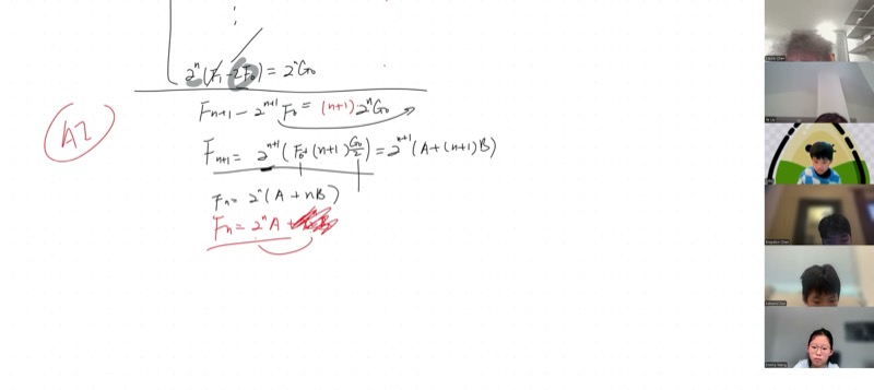
After telescoping \(n+1\) equations, we get:
\[f(n+1) - 2^{n+1} f(0) = (n+1) \cdot 2^n \cdot g(0)\]
Solving for \(f(n+1)\) and re-indexing:
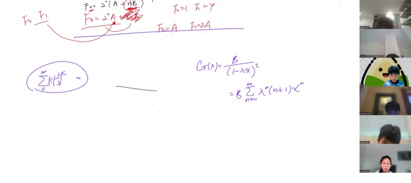
\[\boxed{f(n) = \bigl(A + Bn\bigr) \cdot 2^n}\]
where \(A = f(0)\) and \(B = g(0) = f(1) - 2f(0)\).
Explore the double-root recurrence – change \(f(0)\) and \(f(1)\):
Geometric Series Review
Arithmetic sequence: constant difference \(d\) between terms. \[a_n = a_0 + nd\]
Geometric sequence: constant ratio \(k\) between terms. \[g_n = g_0 \cdot k^n\]
The terms look like: \(g_0,\; g_0 k,\; g_0 k^2,\; g_0 k^3, \ldots\)
The sum of a geometric series (for \(|k| < 1\) in the infinite case):
\[\sum_{n=0}^{\infty} k^n = \frac{1}{1-k}, \qquad |k| < 1\]
For a finite sum:
\[\sum_{n=0}^{N} k^n = \frac{1 - k^{N+1}}{1 - k}\]
Summing Linearly-Scaled Geometric Series
A key result derived in this lecture connects generating functions to our recurrence solution.
\[\frac{1}{(1-x)^2} = \sum_{n=0}^{\infty} (n+1)\,x^n, \qquad |x| < 1\]
This means: \(1 + 2x + 3x^2 + 4x^3 + \cdots = \dfrac{1}{(1-x)^2}\).
We use the generalized binomial theorem: for any real \(\alpha\) and \(|u| < 1\),
\[(1 + u)^\alpha = \sum_{k=0}^{\infty} \binom{\alpha}{k} u^k\]
where the generalized binomial coefficient is:
\[\binom{\alpha}{k} = \frac{\alpha(\alpha-1)(\alpha-2)\cdots(\alpha-k+1)}{k!}\]
Step 1. Write \(\frac{1}{(1-u)^2} = (1 + (-u))^{-2}\).
Step 2. Apply the expansion with \(\alpha = -2\):
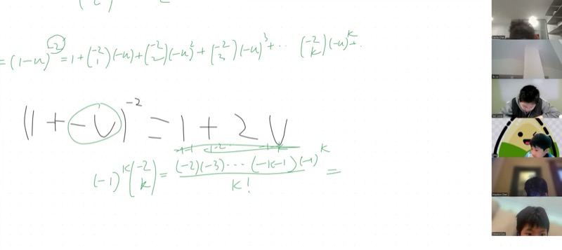
\[(1-u)^{-2} = \sum_{k=0}^{\infty} \binom{-2}{k} (-u)^k\]
Step 3. Compute \(\binom{-2}{k}\):
\[\binom{-2}{k} = \frac{(-2)(-3)(-4)\cdots(-2-k+1)}{k!} = \frac{(-1)^k \cdot (k+1)!}{k!} = (-1)^k(k+1)\]
The numerator has \(k\) terms: \((-2)(-3)\cdots(-(k+1))\). Factoring out \((-1)^k\) gives \(2 \cdot 3 \cdots (k+1) = (k+1)!\).
Step 4. Multiply by \((-u)^k = (-1)^k u^k\):
\[\binom{-2}{k}(-u)^k = (-1)^k(k+1) \cdot (-1)^k u^k = (k+1)\,u^k\]
The \((-1)^k\) factors cancel, giving all positive coefficients.
Result:
\[\frac{1}{(1-u)^2} = \sum_{k=0}^{\infty}(k+1)\,u^k = 1 + 2u + 3u^2 + 4u^3 + \cdots \qquad \blacksquare\]
Worked Example
We want to evaluate \(\sum_{k=1}^{\infty} k \cdot \left(\frac{1}{3}\right)^k\).
Step 1. Factor out \(\frac{1}{3}\):
\[\sum_{k=1}^{\infty} k \left(\frac{1}{3}\right)^k = \frac{1}{3}\sum_{k=1}^{\infty} k \left(\frac{1}{3}\right)^{k-1} = \frac{1}{3}\sum_{j=0}^{\infty} (j+1) \left(\frac{1}{3}\right)^{j}\]
Step 2. Apply our formula with \(x = \frac{1}{3}\):
\[= \frac{1}{3} \cdot \frac{1}{\left(1 - \frac{1}{3}\right)^2} = \frac{1}{3} \cdot \frac{1}{\left(\frac{2}{3}\right)^2} = \frac{1}{3} \cdot \frac{9}{4} = \frac{3}{4}\]
Generating Functions and Partial Fractions
The generating function for a sequence \(\{f(n)\}\) is the power series:
\[G(x) = \sum_{n=0}^{\infty} f(n)\,x^n\]
For a linear recurrence with characteristic roots \(\lambda_1, \lambda_2\), the generating function takes the form:
\[G(x) = \frac{P(x)}{(1 - \lambda_1 x)(1 - \lambda_2 x)}\]
where \(P(x)\) is a polynomial determined by initial conditions.
Distinct roots (\(\lambda_1 \neq \lambda_2\)): Use partial fractions to split:
\[\frac{P(x)}{(1-\lambda_1 x)(1-\lambda_2 x)} = \frac{A}{1-\lambda_1 x} + \frac{B}{1-\lambda_2 x}\]
Each piece expands as a geometric series, giving \(f(n) = A\lambda_1^n + B\lambda_2^n\).
Double root (\(\lambda_1 = \lambda_2 = \lambda\)): The generating function has the form:
\[\frac{A}{1-\lambda x} + \frac{B}{(1-\lambda x)^2}\]
The first piece gives \(A\lambda^n\). The second piece, by our key formula, gives \(B(n+1)\lambda^n\). Combined: \(f(n) = (A + B(n+1))\lambda^n\), which is equivalent to \((A' + B'n)\lambda^n\) after redefining constants.
Explore the partial-fraction decomposition – see how the two pieces combine:
Higher Powers and Pascal’s Triangle
The pattern extends! Using the same binomial expansion technique:
\[\frac{1}{(1-x)^m} = \sum_{n=0}^{\infty} \binom{n+m-1}{m-1} x^n\]
| Power | Coefficients | Name |
|---|---|---|
| \((1-x)^{-1}\) | \(1, 1, 1, 1, \ldots\) | Constant (column 0 of Pascal) |
| \((1-x)^{-2}\) | \(1, 2, 3, 4, \ldots\) | Natural numbers (column 1 of Pascal) |
| \((1-x)^{-3}\) | \(1, 3, 6, 10, \ldots\) | Triangular numbers (column 2 of Pascal) |
| \((1-x)^{-4}\) | \(1, 4, 10, 20, \ldots\) | Tetrahedral numbers (column 3 of Pascal) |
Each column gives the diagonal of Pascal’s triangle! This is because \(\binom{n+m-1}{m-1}\) picks out exactly those entries.
Cheat Sheet
| Concept | Formula / Rule |
|---|---|
| Characteristic equation | \(f(n+1) = pf(n) + qf(n-1) \implies x^2 - px - q = 0\) |
| Distinct roots \(x_1 \neq x_2\) | \(f(n) = Ax_1^n + Bx_2^n\) |
| Double root \(r\) | \(f(n) = (A + Bn)\,r^n\) |
| Geometric series | \(\sum_{n=0}^{\infty} x^n = \frac{1}{1-x}\) for \(|x|<1\) |
| Linearly-scaled geometric | \(\sum_{n=0}^{\infty} (n+1)x^n = \frac{1}{(1-x)^2}\) |
| General negative power | \(\frac{1}{(1-x)^m} = \sum_{n=0}^{\infty}\binom{n+m-1}{m-1}x^n\) |
| Generalized binomial coeff. | \(\binom{\alpha}{k} = \frac{\alpha(\alpha-1)\cdots(\alpha-k+1)}{k!}\) |
| Degrees of freedom | Order-\(k\) recurrence needs \(k\) parameters to match \(k\) initial conditions |