Rational Functions: Horizontal & Slant Asymptotes and the Pitfalls of Infinity
Lecture Video
Key Video Frames
Background
We have previously studied polynomials — finding roots, factoring, and analyzing their behavior as \(x \to \pm\infty\) — as well as completing the square, conic sections, and rotations. Now we take the next step: dividing one polynomial by another to create a rational function. This is exactly the kind of function that appears constantly in pre-calculus and calculus, from modeling real-world phenomena to analyzing rates of change. The central question of this lesson is: what does a rational function look like when \(x\) gets extremely large?
- A rational function is a ratio of two polynomials: \(R(x) = \dfrac{P(x)}{Q(x)}\).
- The asymptotic behavior (what happens as \(x \to \pm\infty\)) depends on comparing the degrees of the numerator and denominator.
- Three cases arise:
- \(\deg(P) = \deg(Q)\): horizontal asymptote at \(y = \dfrac{\text{leading coeff of } P}{\text{leading coeff of } Q}\)
- \(\deg(P) < \deg(Q)\): horizontal asymptote at \(y = 0\)
- \(\deg(P) = \deg(Q) + 1\): slant (oblique) asymptote, found by polynomial long division
- Critical insight: You may discard vanishing terms when the limit is a finite constant, but you must use long division when the limit involves a function of \(x\) (such as a slant asymptote), because vanishing terms on the denominator can shift the result by a nontrivial constant when multiplied back through.
1. Asymptotic Behavior: The Three Cases
Given a rational function \(R(x) = \dfrac{P(x)}{Q(x)}\), we determine its end behavior by comparing the leading terms of the numerator and denominator.
The Simplification Technique
Divide both numerator and denominator by \(x^n\), where \(n\) is the degree of the denominator. Then every term except possibly the leading ones will contain a negative power of \(x\), and those terms approach zero as \(x \to \pm\infty\).
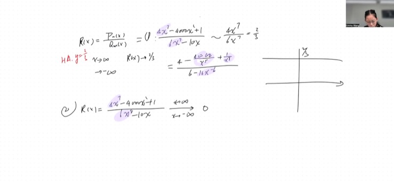
Case 1: Equal Degrees — Horizontal Asymptote
Divide both top and bottom by \(x^7\):
\[R(x) = \frac{4 - \dfrac{4000}{x^5} + \dfrac{1}{x^7}}{6 - \dfrac{10}{x^6}}\]
As \(x \to +\infty\) or \(x \to -\infty\), all the fractional terms approach zero, so:
\[\lim_{x \to \pm\infty} R(x) = \frac{4}{6} = \frac{2}{3}\]
Result: Horizontal asymptote at \(y = \dfrac{2}{3}\).
This shortcut works perfectly here because the final answer is a constant — discarding zeros in the presence of a finite number is completely justified.
Case 2: Denominator Has Higher Degree — Asymptote at Zero
The denominator’s leading term \(6x^8\) dominates the numerator’s \(4x^7\). Even after cancellation, there is a leftover power of \(x\) in the denominator:
\[\frac{4x^7}{6x^8} = \frac{4}{6x} = \frac{2}{3x} \to 0\]
Result: Horizontal asymptote at \(y = 0\) (the \(x\)-axis itself).
The function approaches zero regardless of the sign of \(x\), because the denominator’s power overwhelms the numerator.
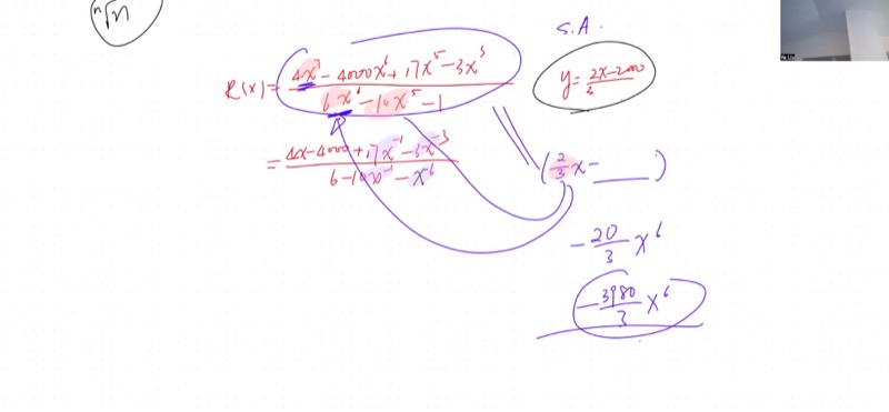
Case 3: Numerator Has Higher Degree — Slant Asymptote
The numerator has degree 7 and the denominator has degree 6. As \(x \to +\infty\), \(R(x) \to +\infty\); as \(x \to -\infty\), \(R(x) \to -\infty\).
The bulk figure suggests the function grows roughly like \(\dfrac{4x^7}{6x^6} = \dfrac{2}{3}x\). But is that really the asymptote?
We must perform polynomial long division to find out. The result is:
\[R(x) = \underbrace{\frac{2}{3}x - \frac{5990}{9}}_{\text{slant asymptote}} + \frac{\text{remainder}}{6x^6 - 10x}\]
The remainder term vanishes as \(x \to \infty\), confirming the slant asymptote is \(y = \dfrac{2}{3}x - \dfrac{5990}{9}\).
Result: The asymptote is NOT simply \(y = \frac{2}{3}x\) — it has an additional constant term revealed only by long division!
Explore the three cases interactively:
2. The Simplification Technique: Dividing by the Leading Power
The standard approach to finding asymptotic behavior:
- Identify the leading power \(x^n\) in the denominator.
- Divide every term in both the numerator and denominator by \(x^n\).
- As \(x \to \pm\infty\), all terms with negative powers of \(x\) approach zero.
- Read off the limit from the remaining non-vanishing terms.
\[R(x) = \frac{4x^7 - 4000x^6 + 17x^5 - 3x^3}{6x^6 - 10x^5 - 1}\]
Divide everything by \(x^6\) (the denominator’s degree):
\[R(x) = \frac{4x - 4000 + 17x^{-1} - 3x^{-3}}{6 - 10x^{-1} - x^{-6}}\]
As \(x \to \infty\), the terms \(17x^{-1}\), \(-3x^{-3}\), \(-10x^{-1}\), and \(-x^{-6}\) all approach zero, so:
\[R(x) \approx \frac{4x - 4000}{6} = \frac{2}{3}x - \frac{2000}{3}\]
Slant asymptote: \(y = \dfrac{2}{3}x - \dfrac{2000}{3}\)
But wait — is this actually correct? The lecture reveals a subtle trap here. Read the next section carefully!
3. The Pitfall: When Can You Discard Vanishing Terms?
This is the deepest insight from the lecture and the one the instructor was most emphatic about.
If the limit is a finite constant (e.g., a horizontal asymptote), you may freely discard terms that approach zero — they are genuinely negligible compared to a fixed number.
If the limit is itself a function that grows without bound (e.g., a slant asymptote like \(\frac{2}{3}x + c\)), you cannot simply discard vanishing terms from the denominator, because when multiplied back through the leading term, they can produce a nontrivial constant contribution.
Why Does This Happen?
Consider the denominator after simplification:
\[6 - 10x^{-1} - x^{-6}\]
The term \(-10x^{-1}\) approaches zero. But in the full expression, the numerator contains a term like \(4x\). When you form the ratio \(\dfrac{4x}{6 - 10x^{-1}}\), the \(-10x^{-1}\) in the denominator interacts with the \(4x\) in the numerator. Expanding:
\[\frac{4x}{6 - 10x^{-1}} \approx \frac{4x}{6}\cdot\frac{1}{1 - \frac{10}{6x}} \approx \frac{2x}{3}\left(1 + \frac{10}{6x} + \cdots\right) = \frac{2x}{3} + \frac{20}{18} + \cdots\]
That “\(\frac{10}{6x}\)” term looked negligible, but multiplied by \(\frac{2x}{3}\), it produced a finite constant \(\frac{10}{9}\) that shifts the asymptote!
Claim: If \(\deg(P) = \deg(Q) + 1\), then \(R(x) = \dfrac{P(x)}{Q(x)} = L(x) + \dfrac{r(x)}{Q(x)}\) where \(L(x) = ax + b\) is the quotient from polynomial long division, \(r(x)\) is the remainder with \(\deg(r) < \deg(Q)\), and the slant asymptote is exactly \(y = L(x)\).
Proof: By the division algorithm for polynomials:
\[P(x) = Q(x) \cdot L(x) + r(x), \quad \deg(r) < \deg(Q)\]
Therefore:
\[R(x) = L(x) + \frac{r(x)}{Q(x)}\]
Since \(\deg(r) < \deg(Q)\), the fraction \(\dfrac{r(x)}{Q(x)} \to 0\) as \(x \to \pm\infty\).
Thus \(R(x) - L(x) \to 0\), which is precisely the definition of \(y = L(x)\) being an asymptote.
The naive method of dividing top and bottom by \(x^n\) can give the correct leading coefficient of \(L(x)\), but it may miss the constant term \(b\) because discarded denominator terms interact with the growing numerator terms to produce that constant.
The General Principle (Beyond Rational Functions)
The instructor stressed that this lesson applies far beyond polynomials:
When simplifying a limit that equals a finite number, discarding terms approaching zero is always safe. When the limit involves a function that grows without bound, discarding “small” terms is dangerous because they can combine with the growing part to produce finite contributions.
This principle will reappear with trigonometric functions, exponential functions, logarithms, and throughout calculus.
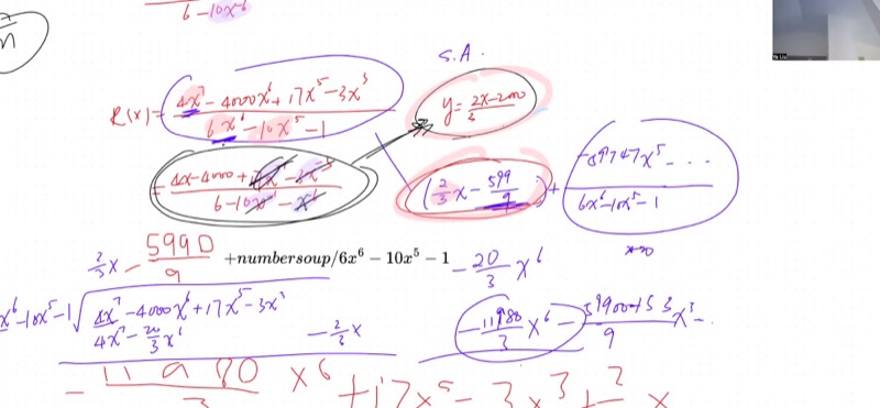
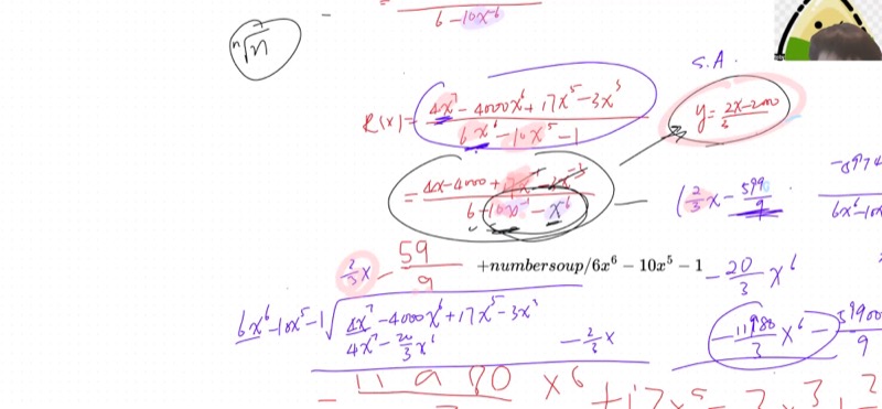
4. Polynomial Long Division: The Reliable Method
When you need exact asymptotic behavior (not just the leading term), long division is required.
Divide \(P(x) = 4x^7 - 4000x^6 + 17x^5 - 3x^3\) by \(Q(x) = 6x^6 - 10x^5 - 1\).
Step 1: Divide leading terms: \(\dfrac{4x^7}{6x^6} = \dfrac{2}{3}x\).
Step 2: Multiply: \(\dfrac{2}{3}x \cdot (6x^6 - 10x^5 - 1) = 4x^7 - \dfrac{20}{3}x^6 - \dfrac{2}{3}x\).
Step 3: Subtract from \(P(x)\):
\[(4x^7 - 4000x^6 + 17x^5 - 3x^3) - (4x^7 - \tfrac{20}{3}x^6 - \tfrac{2}{3}x) = -\frac{11980}{3}x^6 + 17x^5 - 3x^3 + \frac{2}{3}x\]
Step 4: Divide leading terms again: \(\dfrac{-\frac{11980}{3}x^6}{6x^6} = -\dfrac{5990}{9}\).
Step 5: Multiply and subtract to get the remainder.
Result: \(R(x) = \dfrac{2}{3}x - \dfrac{5990}{9} + \dfrac{\text{remainder}}{Q(x)}\)
The slant asymptote is \(y = \dfrac{2}{3}x - \dfrac{5990}{9}\).
Explore long division visually — see how the rational function hugs its slant asymptote:
The blue curve is the rational function. Notice how it approaches the orange dashed line (correct slant asymptote from long division, \(y = 2x - 5\)), not the red dotted line (naive estimate \(y = 2x\)).
5. Summary Table: Finding Asymptotes
| Degree comparison | Asymptote type | How to find it | Method |
|---|---|---|---|
| \(\deg(P) < \deg(Q)\) | Horizontal: \(y = 0\) | Immediate | No division needed |
| \(\deg(P) = \deg(Q)\) | Horizontal: \(y = \dfrac{a_n}{b_n}\) | Divide leading coefficients | Simplify by \(x^n\) |
| \(\deg(P) = \deg(Q) + 1\) | Slant: \(y = mx + b\) | Polynomial long division | Must use long division |
| \(\deg(P) > \deg(Q) + 1\) | No linear asymptote | The function grows too fast | Long division gives a polynomial “asymptote” |
Cheat Sheet
| Question | Answer |
|---|---|
| What is a rational function? | \(R(x) = \dfrac{P(x)}{Q(x)}\), a polynomial divided by a polynomial |
| Horizontal asymptote exists when… | \(\deg(P) \leq \deg(Q)\) |
| Horizontal asymptote value when \(\deg(P) = \deg(Q)\) | \(y = \dfrac{\text{leading coeff of } P}{\text{leading coeff of } Q}\) |
| Slant asymptote exists when… | \(\deg(P) = \deg(Q) + 1\) |
| How to find a slant asymptote | Perform polynomial long division; the quotient \(ax + b\) is the asymptote |
| Can I just divide top/bottom by \(x^n\) for slant asymptotes? | No! This gives only the leading term; you miss the constant shift |
| When is it safe to discard “zero” terms? | When the final answer is a finite constant, not a growing function |
| Approaching from above or below? | Check the sign of the remainder term after long division |
The Principle for Working with Infinity
If your limit is a number, zeros are zeros — discard freely. If your limit is a function of \(x\), vanishing terms can combine with the growing part to produce finite constants. Use long division (or verify by taking the difference).